Polynomial Interpolation
Making your own custom polynomial.
This post is separated into sections based on difficulty. While hopefully anyone with some algebra experience can follow along with the first few sections, the later sections use topics from more advanced math courses like Calculus and Linear Algebra.
When I was just starting to learn algebra, and we were learning about quadratics, I wanted to know how to find a quadratic that passed through certain points. I’ve never been an artist, but the idea of “drawing” a polynomial was novel to me. It wasn’t until college that someone told me how I could do it.
And while I’m perfectly content making up polynomials that look nice just for fun, polynomial interpolation has a number of useful applications. Some of these are:
- Approximating definite integrals of difficult functions by instead integrating an interpolating polynomial
- Filling in values between data points. This can be used to approximate the values of functions like \(\ln(x)\) or the trig functions
- Approximating complicated curves if you only have a few points
And while this is a topic that is occasionally touched on in a linear algebra course, it really only requires relatively basic algebra to get started. If you want to get fancy and creative, then some calculus can spice it up too!
So, let’s try to find a quadratic equation as I wanted to do a long time ago.
I want a quadratic that passes through the points
So we’re looking for a quadratic (degree two) polynomial. The general form of a quadratic is:
\[y=ax^2+bx+c\]However, I’m going to start writing them in a form that generalizes more easily to higher degree polynomials using function notation.
\begin{equation} p(x)=a_0+a_1x+a_2x^2 \end{equation}
There is another reason I do it in this order. It will make solving this problem easier later on (if you use linear algebra).
The first question we must ask ourselves is: “What does it mean for this polynomial to pass through the point \((1,9)\)?”
That may seem like a silly question, and, indeed, when introducing this topic in linear algebra, many students are at a loss for how to even get started with this kind of problem. The key is looking at the point \((x,y)\) with this perspective:
(the input, the output)
And this is where function notation really helps us out. Instead of thinking about the point as \((x,y)\), we want to think about it as
\[(x,p(x))\]In other words, if we want the polynomial to pass through a specific point, we should make sure the desired \(y\) value is produced after plugging in the related \(x\) value. So in the generic case of \((x_1,y_1)\),
\[a_0+a_1x_1+a_2x_1^2=y_1\]which we can also compactly write as \(p(x_1)=y_1\).
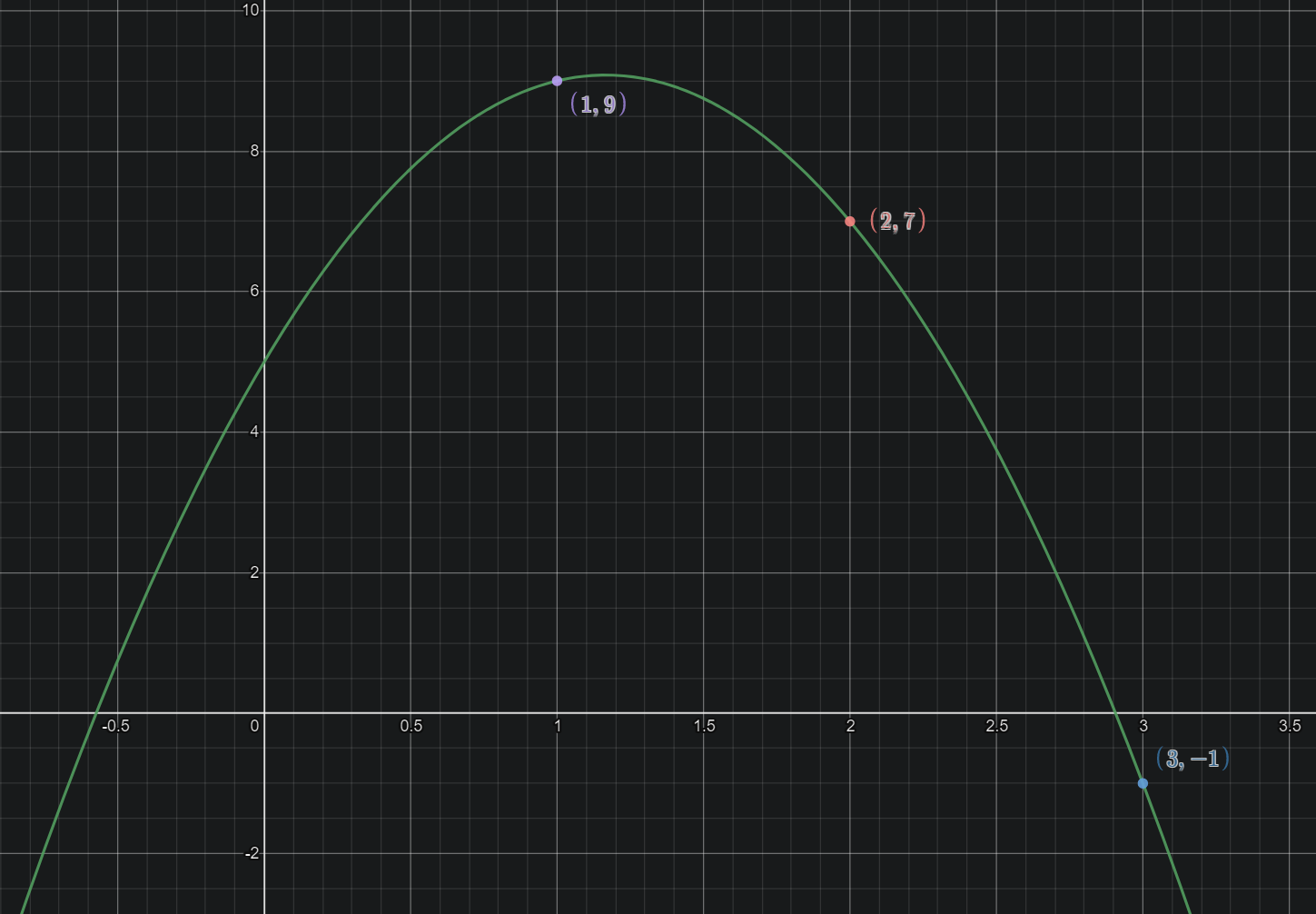
So for each point, we get one equation. In our specific example, \((1,9),(2,7),(3,-1)\), our equations are
\[\begin{align*} a_0+a_1(1)+a_2(1)^2&=9\\ a_0+a_1(2)+a_2(2)^2&=7\\ a_0+a_1(3)+a_2(3)^2&=-1\\ \end{align*}\]Now at this point, we have a system of three equations in three unknowns. Three linear equations at that. Don’t let the \(x^2\) term fool you! Our “variables” are actually the \(a\) coefficients, since it’s those we’re trying to solve for.
Linear algebra can actually tell us that this particular system is guaranteed to have exactly one solution. We will use this idea later to tell us when we are and are not guaranteed a unique polynomial for some given conditions.
It is at this point that I highly recommend writing this in matrix notation so that it’s a lot less cluttered.
\[\begin{equation} \begin{bmatrix} 1&1&1^2\\ 1&2&2^2\\ 1&3&3^2 \end{bmatrix} \begin{bmatrix} a_0\\a_1\\a_2 \end{bmatrix} =\begin{bmatrix} 9\\7\\-1 \end{bmatrix} \end{equation}\]We call the big \(3\times 3\) matrix on the left the “coefficient matrix”. We can do even better, though, by writing it as an “augmented matrix”.
\[\begin{equation} \left[ \begin{array}{ccc|c} 1&1&1^2&9\\ 1&2&2^2&7\\ 1&3&3^2&-1 \end{array} \right] \end{equation}\]Much better right? Now it’s all boiled down to the parts that actually matter: the input points and the output points. We’re basically just skipping the writing of each plus and \(a\) term, and replacing the column of equal signs with a single vertical bar. It’s just a much cleaner way to write it.
That said, if matrix notation is unfamiliar to you, feel free to ignore it! You can solve the systems you get however you like. If you are curious about how to solve systems using matrices and Gaussian elimination in linear algebra, then here is a quick explanation (that you may feel free to skip):
What is Gaussian Elimination? (Click to Expand)
Typically, in linear algebra, one solves these systems using "Gaussian elimination" or "row reduction", which is the same "elimination" method of solving systems of equations taught in earlier algebra courses. As an example of how it works, take the system $$\begin{equation} \begin{array}{ccc} x&+&2y&=&4\\ 2x&+&5y&=&9\\ \end{array} \end{equation}$$ Using elimination we could add -2 of the first equation to the second equation to get rid of the x term. This would give us $$\begin{equation} \begin{array}{cccc} &-2&(&x&+&2y&)&=&-2(4)\\ &+&(&2x&+&5y&)&=&9\\ \hline &&&&&y&&=&1 \end{array} \end{equation}$$ Then our equations become $$\begin{equation} \begin{array}{ccc} x&+&2y&=&4\\ 0x&+&y&=&1\\ \end{array} \end{equation}$$ We can do this with our "agumented matrix" as well. The augmented matrix form of this original system of equations $$\begin{array}{ccc} x&+&2y&=&4\\ 2x&+&5y&=&9\\ \end{array}$$ would be $$\begin{equation} \left[ \begin{array}{cc|c} 1&2&4\\ 2&5&9\\ \end{array} \right] \end{equation}$$ And if we add -2 of the first row to the second (dealing with each column individually), we get $$\left[ \begin{array}{cc|c} 1&2&4\\ 2-2(1)&5-2(2)&9-2(4)\\ \end{array} \right]$$ $$\begin{equation} \left[ \begin{array}{cc|c} 1&2&4\\ 0&1&1\\ \end{array} \right] \end{equation}$$ Giving us $$\begin{array}{ccc} x&+&2y&=&4\\ 0x&+&y&=&1\\ \end{array}$$ as expected. If we add -2 of the new second equation to the first now, then we eliminate the y term in the first. This results in $$\begin{array}{ccc} x&+&0y&=&2\\ 0x&+&y&=&1\\ \end{array}$$ giving us the solution x=2, y=1. In matrix form this is $$\left[ \begin{array}{cc|c} 1&0&2\\ 0&1&1\\ \end{array} \right]$$ As you can see, although Gaussian elimination is no different in practice than regular elimination, it ends up being a lot more compact.A brief aside: If you do choose to solve this with Gaussian elimination, notice how putting the constant term first will make it much easier. It’s natural to instinctively write it with the powers descending, since that’s the standard form of a polynomial, but that just makes it much harder to get the augmented matrix into reduced row echelon form. This way we start with a leading one in the top left corner.
Assuming you were solving it with gaussian elimination, row reducing the matrix yields
\[\begin{equation} \left[ \begin{array}{ccc|c} 1&0&0&5\\ 0&1&0&7\\ 0&0&1&-3 \end{array} \right] \end{equation}\]The way to read this is:
\[\begin{array}{cccc} a_0&&&=&5\\ &a_1&&=&7\\ &&a_2&=&-3\\ \end{array}\]Which should be the result you get by solving the system in whichever way you chose. Here’s a graph of the polynomial \(p(x)=5+7x-3x^2\). As you can see the polynomial does pass through the desired points.
At this point, you can probably figure out most polynomial interpolation problems. Set up your system and solve. However, there are some additional subtleties and ways to make this more general that you may be interested in.
When are we guaranteed a polynomial?
While our first example was a quadratic, let’s turn our attention to the simpler case of two points and a line to get a better intuition for this question. For the purpose of this discussion, we’re going to be assuming that no two points have the same \(x\) value.
If you draw three random points on a piece of paper, can you draw a single straight line through all three? Almost all of the time this is impossible. Not always, however. For example, the three points
\[(1,1),(2,2),(3,3)\]Have a line that passes through them. It’s the line \(y=x\). We call these points “collinear” because they happen to all lie on the same straight line.
By the same logic, if we have four, five, or a hundred points, we aren’t guaranteed a line that passes through all of them unless they happen to be collinear.
Well, how about two points? There is only one line in this situation. In fact we have a formula for it!
\[y=\frac{y_2-y_1}{x_2-x_1}(x-x_1)+y_1\]This next question might seem a bit silly, but if we have just a single point, can we find a line that passes through it?
Well… of course! Take the origin, \((0,0)\), and any line of the form
\[y=mx\]We can pick any number for \(m\) that we like, and, no matter what it is, it will pass through \((0,0)\).
So to recap:
One point: Infinitely many lines
Two points: Exactly one line
Three or more points: There isn’t always a line
So what’s the pattern here? Clearly two points is the special number for a line, but what significance is the number two?
Earlier, I mentioned that linear algebra guaranteed that our system of three equations in three unknowns for our quadratic would have exactly one solution. Three was the magic number for a quadratic, and two seems to be the magic number for a line. Can you spot the pattern?
The equation of a line is
\[p(x)=a_0+a_1x\]And the key is that we have two unknown coefficients, \(a_0\) and \(a_1\). That gives us two degrees of freedom.
Similarly, for a quadratic \(p(x)=a_0+a_1x+a_2x^2\), we have three coefficients, which guarantees us three points since we have three degrees of freedom.
I call these general unknown forms such as \(p(x)=a_0+a_1x\) or \(p(x)=a_0+a_1x+a_2x^2\) the “guess”. It’s an assumption for the form of our solution. And though in real life assumptions are not always correct, in mathematics it can be en exact science to find the correct “guess” or form a solution must take. Without getting too technical, in the case of polynomials like this we are justified in just having the number of \(a_kx^k\) terms in our “guess” be equal to the number of points.
However! Let’s suppose we didn’t realize that the polynomial that passes through \((1,1),(2,2),(3,3)\) is just a line. If we solved it by assuming the answer was of the form \(p(x)=a_0+a_1x+a_2x^2\), we would find that the \(a_2\) coefficient is just zero, giving us the “quadratic” \(p(x)=x\). So just because we have a certain number of points doesn’t mean we know exactly what degree the polynomial will be. But if we assume the number of coefficients is equal to the number of points, we are guaranteed to find exactly one solution.
In summary: The number of points a polynomial can be guaranteed to pass through is equal to the number of unknown coefficients in our guess.
Or in other words: There is exactly one polynomial of degree \(n-1\) or less which passes through \(n\) distinct points.
So if you have five points, for example, that you want a polynomial to pass through, then your guess needs to be a polynomial with five unknown coefficients. Therefore, you need to assume it’s a quartic polynomial.
More creative constraints (Calculus Required)
So far, we’ve been finding polynomials based on points that they pass through. But that’s not the only thing we can guarantee. We’re going to use a bit of calculus for this next section.
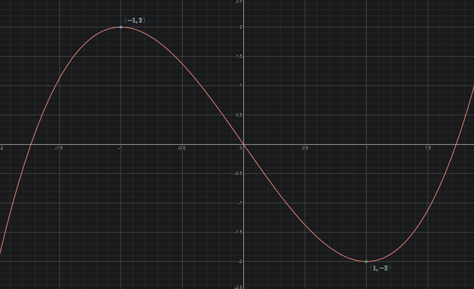
Let’s say we want a polynomial which has a relative maximum at \((-1,2)\) and a relative minimum at \((1,-2)\). Like this.
Calculus tells us that the slope of the tangent line is given by the derivative. So if we want our \(p(x)\) to have a relative maximum or minimum, then we need it’s derivative, \(p'(x)\), to be zero at that point.
So not only do we have the conditions \(p(-1)=2\) and \(p(1)=-2\), but we also need \(p'(-1)=0\) and \(p'(1)=0\).
Since we have four conditions, we need four coefficients. That means a cubic polynomial.
\begin{equation} p(x)=a_0+a_1x+a_2x^2+a_3x^3 \end{equation}
Taking the derivative,
\begin{equation} p’(x)=a_1+2a_2x+3a_3x^2 \end{equation}
And so, our conditions yield us the system of equations
\[\begin{array}{cccc} a_0&+&a_1(-1)&+&a_2(-1)^2&+&a_3(-1)^3&=&2\\ a_0&+&a_1(1)&+&a_2(1)^2&+&a_3(1)^3&=&-2\\ &&a_1&+&2a_2(-1)&+&3a_3(-1)^2&=&0\\ &&a_1&+&2a_2(1)&+&3a_3(1)^2&=&0\\ \end{array}\]In matrix notation, this would be
\[\begin{equation} \left[ \begin{array}{cccc|c} 1&-1&(-1)^2&(-1)^3&2\\ 1&1&1^2&1^3&-2\\ 0&1&2(-1)&3(-1)^2&0\\ 0&1&2(1)&3(1)^2&0 \end{array} \right] \end{equation}\]Now we reduce:
\[\begin{equation} \left[ \begin{array}{cccc|c} 1&0&0&0&0\\ 0&1&0&0&-3\\ 0&0&1&0&0\\ 0&0&0&1&1 \end{array} \right] \end{equation}\] \[\begin{array}{cccc} a_0&&&&=&0\\ &a_1&&&=&-3\\ &&a_2&&=&0\\ &&&a_3&=&1\\ \end{array}\]Thus, our polynomial is \(p(x)=x^3-3x\).
The process of solving was no different than before. The only difference was what our equations looked like. So get creative!
When are we guaranteed a polynomial? Part 2
This section is a bit more technical, and focuses a bit more on the linear algebra aspect of things. Back when we were just discussing points, we only needed the values of \(x_1,\ldots,x_n\) to not be the same, and we would be guaranteed a solution.
This is because our matrix of the form
\[\begin{equation} \begin{bmatrix} 1&x_1&x_1^2&\dots&x_1^{n-1}\\ 1&x_2&x_2^2&\dots&x_2^{n-1}\\ \vdots&\vdots&\vdots&\ddots&\vdots\\ 1&x_n&x_n^2&\dots&x_n^{n-1}\\ \end{bmatrix} \end{equation}\]just so happens to be “invertible” when all the values of \(x_1,\ldots,x_n\) are different. This matrix actually has a special name, too. It is a Vandermonde matrix.
There are a lot of things you can say about a square matrix which is invertible, but some of the most important things for us will be
- If a system of equations has an invertible coefficient matrix, then there is always exactly one unique solution guaranteed.
- If the coefficient matrix of a system is square but not invertible, then there are either no solutions, or infinitely many.
There are a number of tests for invertibility, one computational method being to calculate the determinant. In practice, though, you will discover a matrix is not invertible when you either end up with a free variable or have conflicting equations.
So if we’re just dealing with points, then we don’t have to worry about if we’ll be guaranteed a solution as long as our input points are all different. But, if we start dealing with more complicated constraints, then we will have to be a bit more careful.
An example without a unique solution
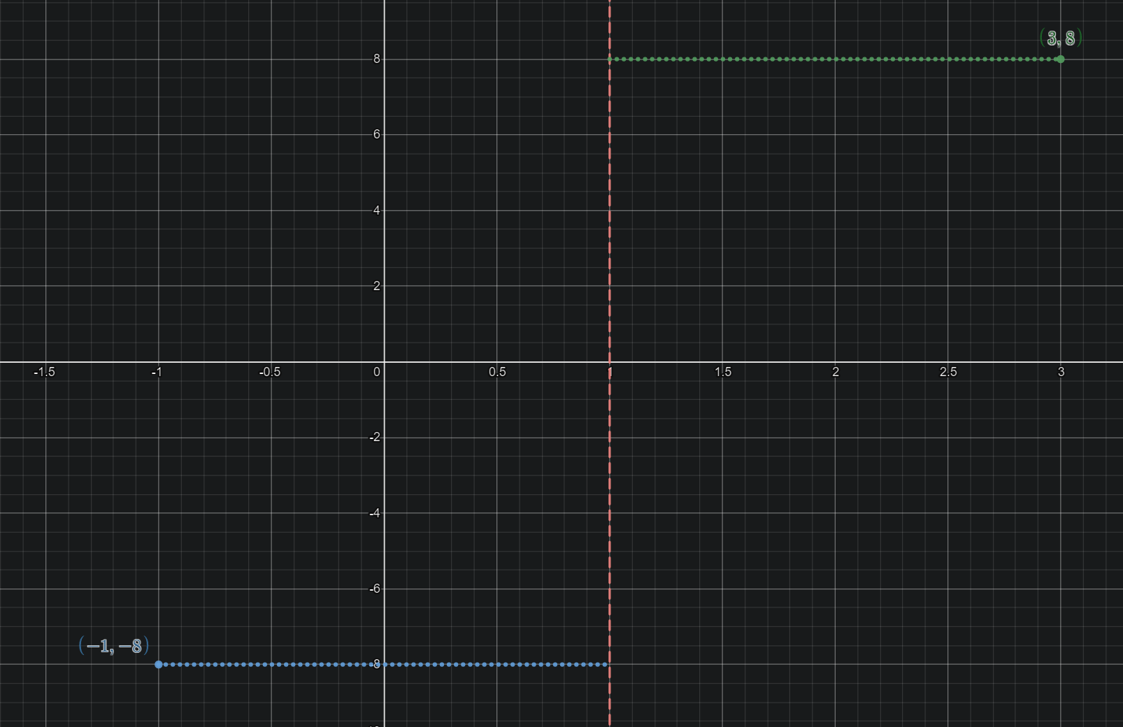
Take the example of wanting a polynomial passing through \((-1,-8)\) and \((3,8)\), while also having a relative extremum at \(x=1\).
Three constraints means three coefficients. So we should be dealing with a quadratic.
\[\begin{array}{cccccc} p(x)&=&a_0&+&a_1x&+&a_2x^2\\ p'(x)&=&&&a_1&+&2a_2x \end{array}\]The constraints give us \(p(-1)=-8,p(3)=8,p'(1)=0\). So our equations will be
\[\begin{array}{cccc} a_0&+&a_1(-1)&+&a_2(-1)^2&=&-8\\ a_0&+&a_1(3)&+&a_2(3)^2&=&8\\ &&a_1&+&2a_2(1)&=&0\\ \end{array}\]Now I recommend trying to solve this system yourself so you can see what happens. But the row reduced version of the matrix form ends up being
\[\begin{equation} \left[ \begin{array}{ccc|c} 1&0&3&0\\ 0&1&2&0\\ 0&0&0&1\\ \end{array} \right] \end{equation}\]Which reads
\[\begin{array}{cccc} a_0&&+&3a_2&=&0\\ &a_1&+&2a_2&=&0\\ &&&0&=&1\\ \end{array}\]Uh-oh. That last equation doesn’t look right. That means there is no solution to this system.
And when you look at it geometrically, that makes sense because no quadratic can possibly make that shape, since they are symmetric about their vertex. Both \(x=-1\) and \(x=3\) are an equal distance from \(x=1\), so any quadratic with a vertex at \(x=1\) will have the same value at \(x=-1\) as it does at \(x=3\).
As a simpler example of this, a quadratic with a vertex at \(x=0\) will look like \(p(x)=ax^2+c\). is it possible for \(p(1)\neq p(-1)\)? No! Because when we plug in \(p(1)\) and \(p(-1)\), we get the exact same output with each, \(p(\pm1)=a+c\).
And indeed, the coefficient matrix
\[\begin{bmatrix} 1&-1&(-1)^2\\ 1&3&(3)^2\\ 0&1&2(1) \end{bmatrix}\]has a determinant of zero. So if we had checked that prior, we would have seen that there would either be no quadratic, or infinitely many which would satisfy our conditions.
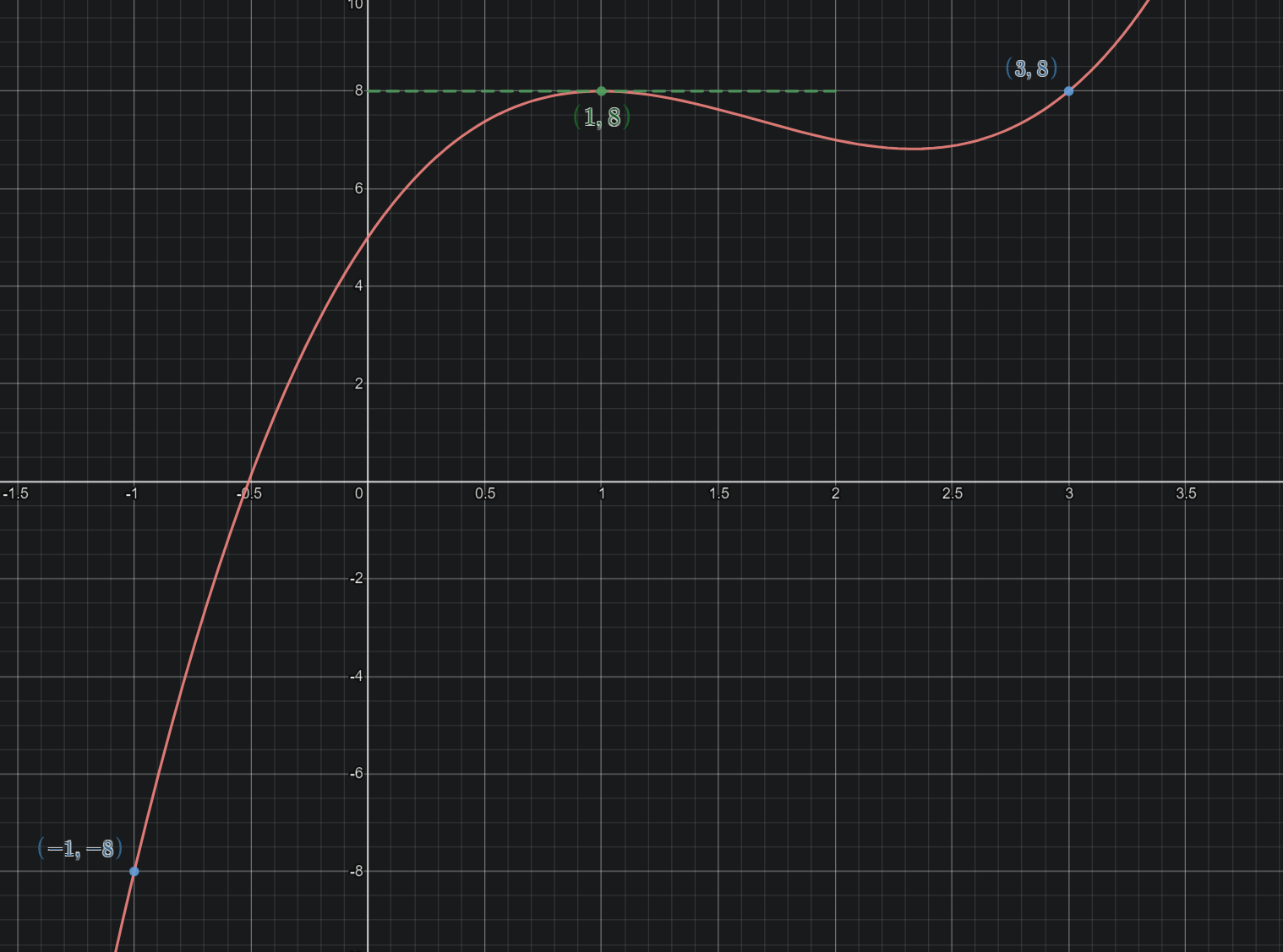
So is all hope lost? For a single unique answer, yes. But there are infinitely many cubics which satisfy our constraints. Specifically, for some number \(t\), any cubic of the form \(\begin{equation} p(x)=x^3-3x-10+t(x^2-2x-3) \end{equation}\)
If you’re wondering how I got that, I just solved the system
\[\begin{array}{cccc} a_0&+&a_1(-1)&+&a_2(-1)^2&+&a_3(-1)^3&=&-8\\ a_0&+&a_1(3)&+&a_2(3)^2&+&a_3(3)^3&=&8\\ &&a_1&+&2a_2(1)&+&3a_3(1)^2&=&0\\ \end{array}\]Now there are plenty of resources that can show you how exactly to solve a system with infinitely many solutions. So instead, I want to point out the conceptual significance the quadratic \(x^2-2x-3\) has to our problem.
\(x^2-2x-3\) has a lot of interesting things going on at \(x\) values of our constraints. The zeros of this quadratic are \(x=-1\) and \(x=3\), and its vertex is at \(x=1\). This is no coincidence!
Because the quadratic is zero at \(x=-1,3\), when we add any scalar multiple of it to our cubic \(x^3-3x-10\), it doesn’t change the value at those points. Since \(x^3-3x-10\) already passes through \((-1,-8)\) and \((3,8)\), then so will \(x^3-3x-10+t(x^2-2x-3)\).
And because both the polynomials \(x^2-2x-3\) and \(x^3-3x-10\) have a relative extremum at \(x=1\), when we add a scalar multiple of the quadratic to the other, the result will still have a relative extremum there. If you know some calculus, I encourage you to try to explain why that is true.
As a final note for this example, we could guarantee a unique solution for a cubic by just adding another requirement. For example, we could specify that \(p(1)=3\), or \(p(x_0)=y_0\) if you want to make it more arbitrary.
My favorite polynomial
This section is more just about some tricks and shortcuts one might use for more complicated polynomials, including a real example which isn’t cherry picked to have a nice answer.
This is the polynomial that I was questing to find when I first learned about polynomial interpolation (purely because it was pretty looking).
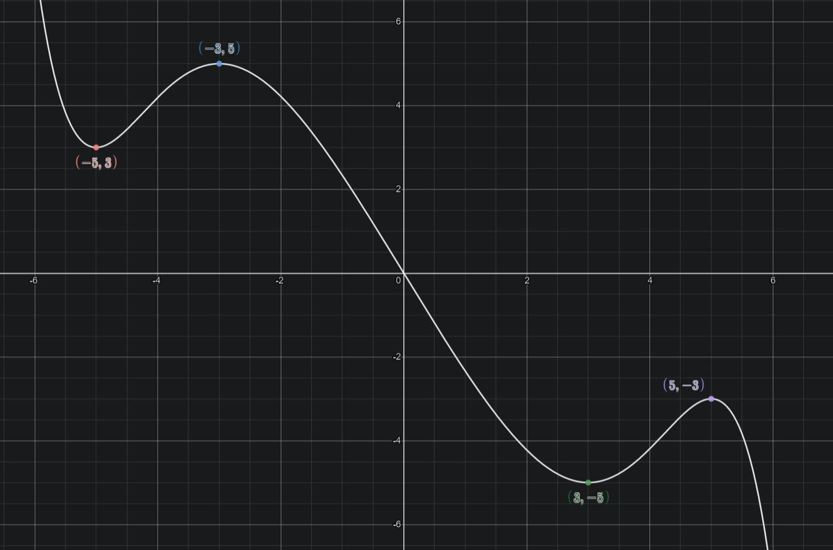
I had drawn the shape and labeled the four points. And while the graph is quite beautiful, the equation itself is not.
In total, the constraints were
\[\begin{array}{cc} p(-5)=3&p'(-5)=0\\ p(-3)=5&p'(-3)=0\\ p(3)=-5&p'(3)=0\\ p(5)=-3&p'(5)=0\\ p(0)=0 \end{array}\]But to find it, I didn’t actually need to set it up with all 9 of these constraints. In fact, I only had to set up four equations!
Instead of doing nine equations, I just noticed that I wanted an odd polynomial. So all the even coefficients \(a_0,a_2,\ldots,a_8\) need to be zero. Since that means it would be mirrored across the origin (including passing through it \(p(0)=0\)), I only needed the constraints \(p(3)=-5,p'(3)=0,p(5)=-3,p'(5)=0\), and the rest would follow from the nature of being odd.
Four constraints, four coefficients. They would all have to be odd though, rather than just being a cubic polynomial. So that would total me up to a degree at most seven polynomial.
My polynomial “guess” was
\[\begin{equation} p(x)=a_1x+a_3x^3+a_5x^5+a_7x^7 \end{equation}\]In summary: if you know that you want your polynomial to satisfy some specific general condition, then make your “guess” reflect that. Similarly, a smart guess can simplify your equations significantly.
As an example of what I mean, in our previous example of having extrema at \((-1,2)\) and \((1,-2)\), if instead of our guess being \(p(x)=a_0+a_1x+a_2x^2+a_3x^3\), we had chosen
\[p(x)=a_0+a_1(x-1)+a_2(x-1)^2+a_3(x-1)^3\]You can verify that two of our equations would be extremely simple. Specifically, the equation for \(p(1)=-2\) is simply \(a_0=-2\), and the equation for \(p'(1)=0\) is just \(a_1=0\). So by making our guess a little strange, we simplified the solving process to really only needing to solve for two variables instead of four. The drawback is that to get our polynomial in standard form we have to expand it out and simplify after solving.
Beyond polynomials
Just like we can set up our “guess” to be an even or odd polynomial, in general, you can use this interpolation method for other types of functions. Our polynomial structure was
\[\begin{equation} p(x)=a_0x^0+a_1x^1+a_2x^2+\ldots+a_{n-1}x^{n-1} \end{equation}\]\(n\) coefficients means \(n\) constraints.
But why limit ourselves to powers of \(x\) on our coefficients?
What if I want a function with exponentials instead of polynomials?
\[\begin{equation} g(x)=a_0e^{0x}+a_1e^{1x}+a_{-1}e^{-1x}+a_2e^{2x}+a_{-2}e^{-2x}+\ldots+a_ne^{nx}+a_{-n}e^{-nx} \end{equation}\]This particular setup would allow me \(2n+1\) constraints.
The process is the same. Plug in your \(g(x_i)\) and set it equal to your desired \(y_i\). The coefficients aren’t quite as pretty, but you’re still just solving a system of equations.
As an example, what if I want a function of the form \(g(x)=a_0+a_1e^{x}+a_{-1}e^{-x}\) that passes through the same points as our original quadratic, \((1,9),(2,7),(3,-1)\). Then my equations will still be
\[\begin{array}{cc} g(1)=9&\implies&a_0+a_1e^{1}+a_{-1}e^{-1}=9\\ g(2)=7&\implies&a_0+a_1e^{2}+a_{-1}e^{-2}=7\\ g(3)=-1&\implies&a_0+a_1e^{3}+a_{-1}e^{-3}=-1\\ \end{array}\] \[\left[ \begin{array}{ccc|c} 1&e^1&e^{-1}&9\\ 1&e^2&e^{-2}&7\\ 1&e^3&e^{-3}&-1\\ \end{array} \right]\]The answer is completely disgusting compared to the simple polynomial we got before, but the graphs look quite similar.
But why even force it to be linear? Why not create a rational function that satisfies \(n+m\) constraints?
\[\begin{equation}\label{rational} g(x)=\frac{a_0+a_1x+\ldots+a_{n-1}x^{n-1}}{b_0+b_1x+\ldots+b_{m-1}x^{m-1}+x^m} \end{equation}\]Since the coefficients of rational functions are based on ratios rather than strict numbers, we can force it to be unique by having what would be \(b_m\) to be \(1\).
Then we can still make it linear by multiplying the denominator to both sides and having our equations be of the form
\[\begin{equation}\label{rationalsys} a_0+a_1x+\ldots+a_{n-1}x^{n-1}-b_0g(x)-b_1xg(x)-\ldots-b_{m-1}x^{m-1}g(x)=x^mg(x) \end{equation}\]For example, let’s say we want a rational function of the form \(g(x)=\frac{a_0}{b_0+b_1x}\) which passes through the points \(\left(-1,\frac{1}{2}\right)\) and \((2,-1)\). Now you may be thinking that we have three unknown coefficients, so we should be able to guarantee three points, right? Well, not quite. Our two equations would be
\[\begin{array}{cc} g(-1)=\frac{1}{2}&\implies&\frac{a_0}{b_0+b_1(-1)}=\frac{1}{2}\\ g(2)=-1&\implies&\frac{a_0}{b_0+b_1(2)}=-1\\ \end{array}\]By multiplying out the denominator to both sides,
\[\begin{array}{cc} a_0&=&\frac{1}{2}(b_0+b_1(-1))\\ a_0&=&-1(b_0+b_1(2))\\ \end{array}\]Getting everything to one side,
\[\begin{array}{cc} a_0&-&\frac{1}{2}b_0&+&\frac{1}{2}b_1&=&0\\ a_0&+&b_0&+&b_1(2)&=&0\\ \end{array}\]This is what we call a “homogeneous” system, since everything on the right side is zero. Homogeneous systems always have at least one solution (one where every unknown is zero, called ‘the trivial solution’), and may have infinitely many. The trivial solution does not work for us, here. It doesn’t make sense for \(g(x)=\frac{0}{0+0x}\). So unless there does happen to be a nontrivial solution for your third point, then you’ll find there is no usable solution.
In this case, there are infinitely many solutions because, as mentioned before, the coefficients on rational functions are based on ratios rather than concrete values. There are infinitely many ways to write a single rational function: \(\frac{a}{bx+c}=\frac{2a}{2bx+2c}\) for example. If we require that \(b_1=1\), then we will actually be guaranteed exactly one unique solution, since our equations could be
\[\begin{array}{cc} a_0&-&\frac{1}{2}b_0&=&-\frac{1}{2}\\ a_0&+&b_0&=&-2\\ \end{array}\]From our general form \eqref{rational}, \(n=1\) and \(m=1\). Our system is indeed in the form \eqref{rationalsys}
\[\begin{array}{cc} a_0&-&b_0g(-1)&=&(-1)^1g(-1)\\ a_0&-&b_0g(2)&=&(2)^1g(2)\\ \end{array}\]The solution to this system is \(a_0=-1,b_0=-1\), so
\[g(x)=-\frac{1}{x-1}\]And here is the graph.
Now solving these problems is considerably more difficult. We no longer have our trusty Vandermonde matrix, and our equations aren’t as pretty, so we have to be more careful in general. We are usually dealing with a lot more constants too, so we have to come up with more constraints if we want a unique solution, and have to solve much larger systems of equations.
That said! It’s possible, and that’s really all that matters, isn’t it?
So for all of you who are inspired, go forth and create beautiful graphs!